Sage as a Calculator¶

This part of the tutorial examines commands that allow you to use Sage much like a graphing calculator. The chapter on arithmetic and functions and the chapter on solving equations and inequalities serve as a foundation for the rest of the material. The chapters on plotting, statistics and calculus are independent of each other, although plotting may be useful to read next since plotting graphs is so is useful in calculus and in statistics.

Arithmetic and Functions¶

Basic Arithmetic¶

The basic arithmetic operators are +, -, *, and / for addition, subtraction, multiplication and division, while ^ is used for exponents.

sage: 1+1
2
sage: 103-101
2
sage: 7*9
63
sage: 7337/11
667
sage: 11/4
11/4
sage: 2^5
32

The - symbol in front of a number indicates that it is negative.

sage: -6
-6
sage: -11+9
-2

As we would expect, Sage adheres to the standard order of operations, PEMDAS (parenthesis, exponents, multiplication, division, addition, subtraction).

sage: 2*4^2+1
33
sage: (2*4)^2+1
65
sage: 2*4^(2+1)
128
sage: -3^2
-9
sage: (-3)^2
9

When dividing two integers, there is a subtlety; whether Sage will return a fraction or it’s decimal approximation. Unlike most graphing calculators, Sage will attempt to be as precise as possible and will return the fraction unless told otherwise. One way to tell Sage that we want the decimal approximation is to include a decimal in the expression itself.

sage: 11/4.0
2.75000000000000
sage: 11/4.
2.75000000000000
sage: 11.0/4
2.75000000000000
sage: 11/4*1.
2.75000000000000

Exercises:

Divide $28$ by $2$ raised to the 5th power as a rational number, then get it’s decimal approximation.

Compute a decimal approximation of $\sqrt{2}$

Use sage to compute (-9)^(1/2). Describe the output.

Integer Division and Factoring¶

You should be familiar with “Basic Arithmetic“

Sometimes when we divide, the division operator doesn’t give us all of the information that we want. Often we would like to not just know what the reduced fraction is, or even it’s decimal approximation, but rather the unique quotient and the remainder that are the consequence of the division.

To calculate the quotient we use the // operator and the % operator is used for the remainder.

sage: 14 // 4
3
sage: 14 % 4
2

If we want both the quotient and the remainder all at once, we use the divmod() command

sage: divmod(14,4)
(3, 2)

Recall that $b$ divides $a$ if $0$ is the remainder when we divide the two integers. The integers in Sage have a built-in command ( or ‘method’ ) which allows us to check whether one integer divides another.

sage: 3.divides(15)
True
sage: 5.divides(17)
False

A related command is the divisors() method. This method returns a list of all positive divisors of the integer specified.

sage: 12.divisors()
[1, 2, 3, 4, 6, 12]
sage: 101.divisors()
[1,101]

When the divisors of an integer are only $1$ and itself then we say that the number is prime. To check if a number is prime in sage, we use it’s is_prime() method.

sage: (2^19-1).is_prime()
True
sage: 153.is_prime()
False

Notice the parentheses around 2^19 -1 in the first example. They are important to the order of operations in Sage, and if they are not included then Sage will compute something very different than we intended. Try evaluating 2^19-1.is_prime() and notice the result. When in doubt, the judicious use of parenthesis is encouraged.

We use the factor() method to compute the prime factorization of an integer.

sage: 62.factor()
2 * 31
sage: 63.factor()
3^2 * 7

If we are interested in simply knowing which prime numbers divide an integer, we may use it’s prime_divisors() (or prime_factors()) method.

sage: 24.prime_divisors()
[2, 3]
sage: 63.prime_factors()
[3, 7]

Finally, we have the greatest common divisor and least common multiple of a pair of integers. A common divisor of two integers is any integer which is a divisor of each, whereas a common multiple is a number which both integers divide.

The greatest common divisor (gcd), not too surprisingly, is the largest of all of these common divisors. The gcd() command is used to calculate this divisor.

sage: gcd(14,63)
7
sage: gcd(15,19)
1

Notice that if two integers share no common divisors, then their gcd will be $1$ .

The least common multiple is the smallest integer which both integers divide. The lcm() command is used to calculate the least common multiple.

sage: lcm(4,5)
20
sage: lcm(14,21)
42

Exercises:

Find the quotient and remainder when diving $98$ into $956$ .

Use Sage to verify that the quotient and remainder computed above are correct.

Use Sage to determine if $3$ divides $234878$ .

Compute the list of divisors for each of the integers $134,\ 491,\ 422$ and $1002$ .

Which of the integers above are prime?

Calculate $\mathrm{gcd}(a,b)$ , $\mathrm{lcm}(a,b)$ and $a \cdot b$ for the pairs of integers $\left(2,5\right),\ \left(4,10\right)$ and $\left(18,51\right)$ . How do the gcd, lcm and the product of the numbers relate?

Standard Functions and Constants¶

Sage includes nearly all of the standard functions that one encounters when studying mathematics. In this section, we shall cover some of the most commonly used functions: the maximum, minimum, floor, ceiling, trigonometric, exponential, and logarithm functions. We will also see many of the standard mathematical constants; such as Euler’s constant ( $e$ ), $\pi$ , and the golden ratio ( $\phi$ ).

The max() and min() commands return the largest and smallest of a set of numbers.

sage: max(1,5,8)
8
sage: min(1/2,1/3)
1/3

We may input any number of arguments into the max and min functions.

In Sage we use the abs() command to compute the absolute value of a real number.

sage: abs(-10)
10
sage: abs(4)
4

The floor() command rounds a number down to the nearest integer, while ceil() rounds up.

sage: floor(2.1)
2
sage: ceil(2.1)
3

We need to be very careful while using floor() and ceil().

sage: floor(1/(2.1-2))
9

This is clearly not correct: $\lfloor 1/(2.1-2)\rfloor = \lfloor 1/.1 \rfloor = \lfloor 10 \rfloor = 10$ . So what happened?

sage: 1/(2.1-2)
9.99999999999999

Computers store real numbers in binary, while we are accustomed to using the decimal representation. The $2.1$ in decimal notation is quite simple and short, but when converted to binary it is $10.0001\overline{1}=10.0001100110011\ldots$

Since computers cannot store an infinite number of digits, this gets rounded off somewhere, resulting in the slight error we saw. In Sage, however, rational numbers (fractions) are exact, so we will never see this rounding error.

sage: floor(1/(21/10-2))
10

Due to this, it is often a good idea to use rational numbers whenever possible instead of decimals, particularly if a high level of precision is required.

The sqrt() command calculates the square root of a real number. As we have seen earlier with fractions, if we want a decimal approximation we can get this by giving a decimal number as the input.

sage: sqrt(3)
sqrt(3)
sage: sqrt(3.0)
1.73205080756888

To compute other roots, we use a rational exponent. Sage can compute any rational power. If either the exponent or the base is a decimal then the output will be a decimal.

sage: 3^(1/2)
sqrt(3)
sage: (3.0)^(1/2)
1.73205080756888
sage: 8^(1/2)
2*sqrt(2)
sage: 8^(1/3)
2

Sage also has available all of the standard trigonometric functions: for sine and cosine we use sin() and cos().

sage: sin(1)
sin(1)
sage: sin(1.0)
0.841470984807897
sage: cos(3/2)
cos(3/2)
sage: cos(3/2.0)
0.0707372016677029

Again we see the same behavior that we saw with sqrt(), Sage will give us an exact answer. You might think that since there is no way to simplify sin(1), why bother? Well, some expressions involving sine can indeed be simplified. For example, an important identity from geometry is $\sin(\pi/3 ) = \sqrt{3}/2$ . Sage has a built-in symbolic $\pi$ , and understands this identity:

sage: pi
pi
sage: sin(pi/3)
1/2*sqrt(3)

When we type pi in Sage we are dealing exactly with $\pi$ , not some numerical approximation. However, we can call for a numerical approximation using the n() method:

sage: pi.n()
3.14159265358979
sage: sin(pi)
0
sage: sin(pi.n())
1.22464679914735e-16

We see that when using the symbolic pi, Sage returns the exact result. However, when we use the approximation we get an approximation back. e-15 is a shorthand for $10^{-15}$ and the number 1.22464679914735e-16 should be zero, but there are errors introduced by the approximation. Here are a few examples of using the symbolic, precise $\pi$ vs the numerical approximation:

sage: sin(pi/6)
1/2
sage: sin(pi.n()/6)
0.500000000000000
sage: sin(pi/4)
1/2*sqrt(2)
sage: sin(pi.n()/4)
0.707106781186547

Continuing on with the theme, there are some lesser known special angles for which the value of sine or cosine can be cleverly simplified.

sage: sin(pi/10)
1/4*sqrt(5) - 1/4
sage: cos(pi/5)
1/4*sqrt(5) + 1/4
sage: sin(5*pi/12)
1/12*(sqrt(3) + 3)*sqrt(6)

Other trigonometric functions, the inverse trigonometric functions and hyperbolic functions are also available.

sage: arctan(1.0)
0.785398163397448
sage: sinh(9.0)
4051.54190208279

Similar to pi Sage has a built-in symbolic constant for the number $e$ , the base of the natural logarithm.

sage: e
e
sage: e.n()
2.71828182845905

While some might be familiar with using ln(x) for natural log and log(x) to represent logarithm base $10$ , in Sage both represent logarithm base $e$ . We may specify a different base as a second argument to the command: to compute $\log_{b}(x)$ in Sage we use the command log(x,b).

sage: ln(e)
1
sage: log(e)
1
sage: log(e^2)
2
sage: log(10)
log(10)
sage: log(10.0)
2.30258509299405
sage: log(100,10)
2

Exponentiation base $e$ can done using both the exp() function and by raising the symbolic constant e to a specified power.

sage: exp(2)
e^2
sage: exp(2.0)
7.38905609893065
sage: exp(log(pi))
pi
sage: e^(log(2))
2

Exercises:

Compute the floor and ceiling of $2.75$ .

Compute the logarithm base $e$ of $1/1000000$ , compute the logarithm base 10 of $1/1000000$ , then compute the ratio. What should the answer be?

Compute the logarithm base 2 of $64$ .

Compare $e^{i \pi}$ with a numerical approximation of it using pi.n().

Compute $\sin(\pi/2)$ , $\cot(0)$ and $\csc(\pi/16)$ .

Solving Equations and Inequalities¶

Solving for x¶

You should be familiar with “Basic Arithmetic” and “Standard Functions and Constants“

In Sage, equations and inequalities are defined using the operators ==, <=, and >= and will return either True, False, or, if there is a variable, just the equation/inequality.

sage: 9 == 9
True
sage: 9 <= 10
True
sage: 3*x - 10 == 5
3*x - 10 == 5

To solve an equation or an inequality we use using the, aptly named, solve() command. For the moment, we will only solve for $x$ . The section on variables below explains how to use other variables.

sage: solve(3*x - 2 == 5,x)
[x == (7/3)]
sage: solve( 2*x -5 == 1, x)
[x == 3]
sage: solve( 2*x - 5 >= 17,x)
[[x >= 11]]
sage: solve( 3*x -2 > 5, x)
[[x > (7/3)]]

Equations can have multiple solutions, Sage returns all solutions found as a list.

sage: solve( x^2 + x  == 6, x)
[x == -3, x == 2]
sage: solve(2*x^2 - x + 1 == 0, x)
[x == -1/4*I*sqrt(7) + 1/4, x == 1/4*I*sqrt(7) + 1/4]
sage: solve( exp(x) == -1, x)
[x == I*pi]

The solution set of certain inequalities consists of the union and intersection of open intervals.

sage: solve( x^2 - 6 >= 3, x )
[[x <= -3], [x >= 3]]
sage: solve( x^2 - 6 <= 3, x )
[[x >= -3, x <= 3]]

The solve() command will attempt to express the solution of an equation without the use of floating point numbers. If this cannot be done, it will return the solution in a symbolic form.

sage: solve( sin(x) == x, x)
[x == sin(x)]
sage: solve( exp(x) - x == 0 , x)
[x == e^x]
sage: solve( cos(x) - sin(x) == 0 , x)
[sin(x) == cos(x)]
sage: solve( cos(x) - exp(x) == 0 , x)
[cos(x) == e^x]

To find a numeric approximation of the solution we can use the find_root() command. Which requires both the expression and a closed interval on which to search for a solution.

sage: find_root(sin(x) == x, -pi/2 , pi/2)
0.0
sage: find_root(sin(x) == cos(x), pi, 3*pi/2)
3.9269908169872414

This command will only return one solution on the specified interval, if one exists. It will not find the complete solution set over the entire real numbers. To find a complete set of solutions, the reader must use find_root() repeatedly over cleverly selected intervals. Sadly, at this point, Sage cannot do all of the thinking for us. This feature is not planned until Sage 10.

Declaring Variables¶

In the previous section we only solved equations in one variable, and we always used $x$ . When a session is started, Sage creates one symbolic variable, $x$ , and it can be used to solve equations. If you want to use an additional symbolic variable, you have to declare it using the var() command. The name of a symbolic variable can be a letter, or a combination of letters and numbers:

sage: y,z,t = var("y z t")
sage: phi, theta, rho = var("phi theta rho")
sage: x1, x2 = var("x1 x2")

Note

Variable names cannot contain spaces, for example “square root” is not a valid variable name, whereas “square_root” is.

Attempting to use a symbolic variable before it has been declared will result in a NameError.

sage: u
...
NameError: name 'u' is not defined
sage: solve (u^2-1,u)
NameError                                 Traceback (most recent call last)
NameError: name 'u' is not defined

We can un-declare a symbolic variable, like the variable phi defined above, by using the restore() command.

sage: restore('phi')
sage: phi
...
NameError: name 'phi' is not defined

Solving Equations with Several Variables¶

Small systems of linear equations can be also solved using solve(), provided that all the symbolic variables have been declared. The equations must be input as a list, followed by the symbolic variables. The result may be either a unique solution, infinitely many solutions, or no solutions at all.

sage: solve( [3*x - y == 2, -2*x -y == 1 ], x,y)
[[x == (1/5), y == (-7/5)]]
sage: solve( [  2*x + y == -1 , -4*x - 2*y == 2],x,y)
[[x == -1/2*r1 - 1/2, y == r1]]
sage: solve( [  2*x - y == -1 , 2*x - y == 2],x,y)
[]

In the second equation above, r1 signifies that there is a free variable which parametrizes the solution set. When there is more than one free variable, Sage enumerates them r1,r2,..., rk.

sage: solve([ 2*x + 3*y + 5*z == 1, 4*x + 6*y + 10*z == 2, 6*x + 9*y + 15*z == 3], x,y,z)
[[x == -5/2*r1 - 3/2*r2 + 1/2, y == r2, z == r1]]

solve() can be very slow for large systems of equations. For these systems, it is best to use the linear algebra functions as they are quite efficient.

Solving inequalities in several variables can lead to complicated expressions, since the regions they define are complicated. In the example below, Sage’s solution is a list containing the point of interesection of the lines, then two rays, then the region between the two rays.

sage: solve([ x-y >=2, x+y <=3], x,y)
[[x == (5/2), y == (1/2)], [x == -y + 3, y < (1/2)], [x == y + 2, y < (1/2)], [y + 2 < x, x < -y + 3, y < (1/2)]]
sage: solve([ 2*x-y< 4, x+y>5, x-y<6], x,y)
[[-y + 5 < x, x < 1/2*y + 2, 2 < y]]

Exercises:

Find all of the solutions to the equation $x^3 - x = 7x^2 - 7$ .

Find the complete solution set for the inequality $\left\vert t - 7 \right\vert \geq 3$ .

Find all $x$ and $y$ that satisfy both $2x + y = 17$ and $x - 3y = -16$ .

Use find_root() to find a solution of the equation $e^{x} = \cos(x)$ on the interval $\left[-\pi/2, 0\right]$ .

Change the command above so that find_root() finds the other solution in the same interval.

Calculus¶

You should be familiar with Basic Arithmetic, Standard Functions and Constants, and Declaring Variables

Sage has many commands that are useful for the study of differential and integral calculus. We will begin our investigation of these command by defining a few functions that we will use throughout the chapter.

sage: f(x) = x*exp(x)
sage: f
x |--> x*e^x
sage: g(x) = (x^2)*cos(2*x)
sage: g
x |--> x^2*cos(2*x)
sage: h(x) = (x^2 + x - 2)/(x-4)
sage: h
x |--> (x^2 + x - 2)/(x-4)

Sage uses x |--> to tell you that the expression returned is actually a function and not just a number or string. This means that we can evaluate these expressions just like you would expect of any function.

sage: f(1)
e
sage: g(2*pi)
4*pi^2
sage: h(-1)
2/5

With these functions defined, we will look at how we can use Sage to compute the limit of these functions.

Limits¶

The limit of $f(x) = xe^{x}$ as $x \rightarrow 1$ is computed in Sage by entering the following command into Sage:

sage: limit(f, x=1)
e

We can do the same with $g(x)$ . To evaluate the limit of $g(x) = x^{2} \cos(2x)$ as $x \rightarrow 2$ we enter:

sage: limit(g, x=2)
4*cos(4)

The functions $f(x)$ and $g(x)$ aren’t all that exciting as far as limits are concerned since they are both continuous for all real numbers. But $h(x)$ has a discontinuity at $x=4$ , so to investigate what is happening near this discontinuity we will look at the limit of $h(x)$ as $x \rightarrow 4$ :

sage: limit(h, x = 4)
Infinity

Now this is an example of why we have to be a little careful when using computer algebra systems. The limit above is not exactly correct. See the graph of $h(x)$ near this discontinuity below.

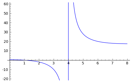
"Rational Function with vertical asymptote x=4"

What we have when $x=4$ is a vertical asymptote with the function tending toward positive infinity if $x$ is larger than $4$ and negative infinity from when $x$ less than $4$ . We can takes these directional limits using Sage to confirm this by supplying the extra dir argument.

sage: limit(h, x=4, dir="right")
+Infinity
sage: limit(h, x=4, dir="left")
-Infinity

Derivatives¶

The next thing we are going to do is use Sage to compute the derivatives of the functions that we defined earlier. For example, to compute $f^{\prime}(x)$ , $g^{\prime}(x)$ , and $h^{\prime}(x)$ we will use the derivative() command.

sage: fp  =  derivative(f,x)
sage: fp
x |--> x*e^x + e^x
sage: gp =  derivative(g, x)
sage: gp
x |--> -2*x^2*sin(2*x) + 2*x*cos(2*x)
sage: hp  = derivative(h,x)
sage: hp
x |--> (2*x + 1)/(x - 4) - (x^2 + x - 2)/(x - 4)^2

The first argument is the function which you would like to differentiate and the second argument is the variable with which you would like to differentiate with respect to. For example, if I were to supply a different variable, Sage will hold $x$ constant and take the derivative with respect to that variable.

sage: y = var('y')
sage: derivative(f,y)
x |--> 0
sage: derivative(g,y)
x |--> 0
sage: derivative(h,y)
x |--> 0

The derivative() command returns another function that can be evaluated like any other function.

sage: fp(10)
11*e^10
sage: gp(pi/2)
-pi
sage:
sage: hp(10)
1/2

With the derivative function computed, we can then find the critical points using the solve() command.

sage: solve( fp(x) == 0, x)
[x == -1, e^x == 0]
sage: solve( hp(x) == 0, x)
[x == -3*sqrt(2) + 4, x == 3*sqrt(2) + 4]
sage: solve( gp(x) == 0, x)
[x == 0, x == cos(2*x)/sin(2*x)]

Constructing the line tangent to our functions at the point $\left(x, f\left(x\right)\right)$ is an important computation which is easily done in Sage. For example, the following command will compute the line tangent to $f(x)$ at the point $\left(0,f(0)\right)$ .

sage: T_f = fp(0)*( x - 0 ) + f(0)
sage: T_f
x

The same can be done for $g(x)$ and $h(x)$ .

sage: T_g = gp(0)*( x - 0 ) + g(0)
sage: T_g
0
sage: T_h = hp(0)*( x - 0 ) + h(0)
sage: T_h
-1/8*x + 1/2

Integrals¶

Sage has the facility to compute both definite and indefinite integral for many common functions. We will begin by computing the indefinite integral, otherwise known as the anti-derivative, for each of the functions that we defined earlier. This will be done by using the integral() command which has arguments that are similar to derivative().

sage: integral(f,x)
x |--> (x - 1)*e^x
sage: integral(g, x)
x |--> 1/4*(2*x^2 - 1)*sin(2*x) + 1/2*x*cos(2*x)
sage: integral(h, x)
x |--> 1/2*x^2 + 5*x + 18*log(x - 4)

The function that is returned is only one of the many anti-derivatives that exist for each of these functions. The others differ by a constant. We can verify that we have indeed computed the anti-derivative by taking the derivative of our indefinite integrals.

sage: derivative(integral(f,x), x )
x |--> (x - 1)*e^x + e^x
sage: f
x |--> x*e^x
sage: derivative(integral(g,x), x )
x |--> 1/2*(2*x^2 - 1)*cos(2*x) + 1/2*cos(2*x)
sage: derivative(integral(h,x), x )
x |--> x + 18/(x - 4) + 5

Wait, none of these look right. But a little algebra, and the use of a trig-identity or two in the case of 1/2*(2*x^2 - 1)*cos(2*x) + 1/2*cos(2*x), you will see that they are indeed the same.

It should also be noted that there are some functions which are continuous and yet there doesn’t exist a closed form integral. A common example is $e^{-x^2}$ which forms the basis for the normal distribution which is ubiquitous throughout statistics. The antiderivative for $er^{-x^2}$ is commonly called $\mathrm{erf}$ , otherwise known as the error function.

sage: y(x) = exp(-x^2)
sage: integral(y,x)
x |--> 1/2*sqrt(pi)*erf(x)

We can also compute the definite integral for the functions that we defined earlier. This is done by specifying the limits of integration as addition arguments.

sage: integral(f, x,0,1)
x |--> 1
sage: integral(g,x,0,1)
x |--> 1/4*sin(2) + 1/2*cos(2)
sage: integral(h, x,0,1)
x |--> 18*log(3) - 18*log(4) + 11/2

In each case above, Sage returns a function as its result. Each of these functions is a constant function, which is what we would expect. As it was pointed out earlier, Sage will return the expression that retains the most precision and will not use decimals unless told to. A quick way to tell Sage that an approximation is desired is wrap the integrate() command with n(), the numerical approximation command.

sage: n(integral(f, x,0,1))
1.00000000000000
sage: n(integral(g, x,0,1))
0.0192509384328492
sage: n(integral(h, x,0,1))
0.321722695867944

Exercises:

Use Sage to compute the following limits:

$\lim_{x \rightarrow 2} \frac{x^{2} + 2 \, x - 8}{x-2}$

$\lim_{x \rightarrow (\pi/2)^{+}} \sec(x)$

$\lim_{x \rightarrow (\pi/2)^{-}} \sec(x)$

Use Sage to compute the following derivatives with respect to the specified variables:

$\frac{d}{dx}\left[ x^{2}e^{3x}\cos(2x) \right]$

$\frac{d}{dt}\left[\frac{t^2 + 1}{t-2}\right]$ (remember to define ``t``)

$\frac{d}{dy}\left[ x\cos(x)\right]$

Use Sage to compute the following integrals:

$\int \frac{x+1}{x^2 + 2x + 1}dx$

$\int_{-\pi/4}^{\pi/4} \sec(x) dx$

$\int x e^{-x^{2}} dx$

Statistics¶

You should be familiar with Basic Arithmetic

In this section we will discuss the use of some of the basic descriptive statistic functions availble for use in Sage.

To demonstrate their usage we will first generate a pseudo-random list of integers to describe. The random() function generates a random number from $[0,1)$ , so we will use a trick. Note, by the nature of random number generation your list of numbers will be different.

sage: data = [  floor(tan( pi* random() - pi/2.1 )) for i in [ 1 .. 20 ] ]
sage: data
[1, -1, -7, 0, -4, -1, -2, 1, 3, 5, -1,
25, -5, 1, 2, 0, 1, -1, -1, -1]

We can compute the mean, median, mode, variance, and standard deviation of this data.

sage: mean(data)
3/4
sage: median(data)
-1/2
sage: mode(data)
[-1]
sage: variance(data)
3023/76
sage: std(data)
1/2*sqrt(3023/19)

Note that both the standard deviation and variance are computed in their unbiased forms. It we want to bias these measures then you can use the bias=True option.

We can also compute a rolling, or moving, average of the data with the moving_average().

sage: moving_average(data,4)
[-7/4, -3, -3, -7/4, -3/2, 1/4, 7/4, 2, 8, 6, 5, 23/4,
-1/2, 1, 1/2, -1/4, -1/2]
sage: moving_average(data,10)
[-1/2, -7/10, 19/10, 21/10, 11/5, 14/5, 29/10, 16/5, 3, 13/5, 2]
sage: moving_average(data,20)
[3/4]

Exercises:

Use Sage to generate a list of 20 random integers.

The heights of eight students, measured in inches, are $71,\ 73,\ 59,\ 62,\ 65,\ 61,\ 73,\ 61$ . Find the average, median and mode of the heights of these students.

Using the same data, compute the standard deviation and variance of the sampled heights.

Find the range of the heights. (Hint: use the max() and min() commands)

Plotting¶

2D Graphics¶

You should be familiar with Standard Functions and Constants and Solving Equations and Inequalities

Sage has many ways for us to visualize the mathematics with which we are working. In this section we will quickly you up to speed with some of the basic commands used when plotting functions and working with graphics.

To produce a basic plot of $\sin(x)$ from $x=-\frac{\pi}{2}$ to $x=\frac{\pi}{2}$ we will use the plot() command.

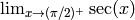
sage: f(x) = sin(x)
sage: p = plot(f(x), (x, -pi/2, pi/2))
sage: p.show()

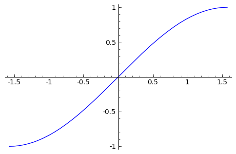
By default, the plot created will be quite plain. To add axis labels and make our plotted line purple, we can alter the plot attribute by adding the axes_labels and color options.

sage: p = plot(f(x), (x,-pi/2, pi/2), axes_labels=['x','sin(x)'], color='purple')
sage: p.show()

Plot of sin with purple line and basic axis labels

The color option accepts string color designations ( ‘purple’, ‘green’, ‘red’, ‘black’, etc...), an RGB triple such as (.25,.10,1), or an HTML-style hex triple such as #ff00aa.

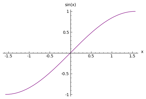
We can change the style of line, whether it is solid, dashed, and it’s thickness by using the linestyle and the thickness options.

sage: p = plot(f(x), (x,-pi/2, pi/2), linestyle='--', thickness=3)
sage: p.show()

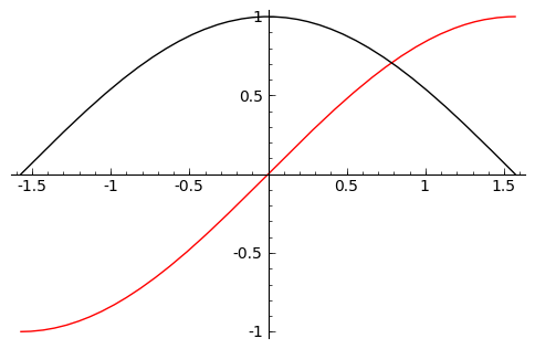
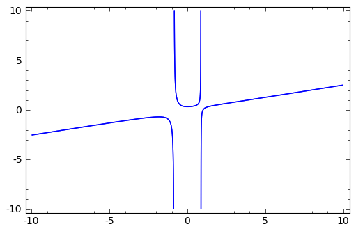
Plot of sin(x) using a thick dashed blue line

We can display the graphs of two functions on the same axes by adding the plots together.

sage: f(x) = sin(x)
sage: g(x) = cos(x)
sage: p = plot(f(x),(x,-pi/2,pi/2), color='black')
sage: q = plot(g(x), (x,-pi/2, pi/2), color='red')
sage: r = p + q
sage: r.show()

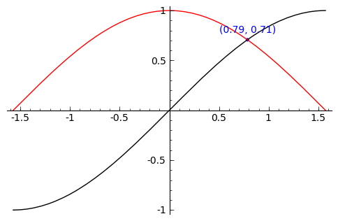
Plot of sin(x) and cos(x) on the same axes

To tie together our plotting commands with some material we have learned earlier, let’s use the find_root() command to find the point where $\sin(x)$ and $\cos(x)$ intersect. We will then add this point to the graph and label it.

sage: find_root( sin(x) == cos(x),-pi/2, pi/2 )
0.78539816339744839
sage: P = point( [(0.78539816339744839, sin(0.78539816339744839))] )
sage: T = text("(0.79,0.71)", (0.78539816339744839, sin(0.78539816339744839) + .10))
sage: s = P + r + T
sage: s.show()

sin(x) and cos(x) on same axes with point of intersection labeled

Sage handles many of the details of producing “nice” looking plots in a way that is transparent to the user. However there are times in which Sage will produce a plot which isn’t quite what we were expecting.

sage: f(x) = (x^3 + x^2 + x)/(x^2 - x -2 )
sage: p = plot(f(x), (x, -5,5))
sage: p.show()

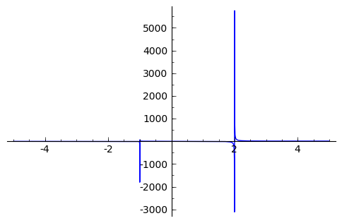
Plot of rational function with asymptotes

The vertical asymptotes of this rational function cause Sage to adjust the aspect ratio of the plot to display the rather large $y$ values near $x=-1$ and $x=2$ . This obfuscates most of the features of this function in a way that we may have not intended. To remedy this we can explicitly adjust the vertical and horizontal limits of our plot

sage: p.show(xmin=-2, xmax=4, ymin=-20, ymax=20)

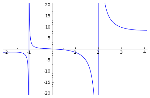
Plot of rational function with asymptote with vertical limits adjusted

This, in the author’s opinion, displays the features of this particular function in a much more pleasing fashion.

Sage can handle parametric plots with the parametric_plot() command. The following is a simple circle of radius 3.

sage: t = var('t')
sage: p = parametric_plot( [3*cos(t), 3*sin(t)], (t, 0, 2*pi) )
sage: p.show()

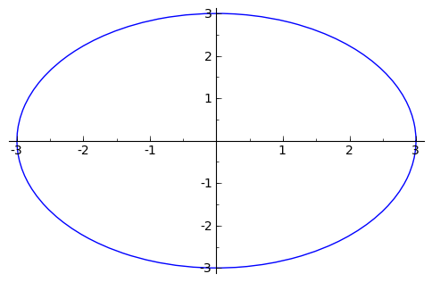
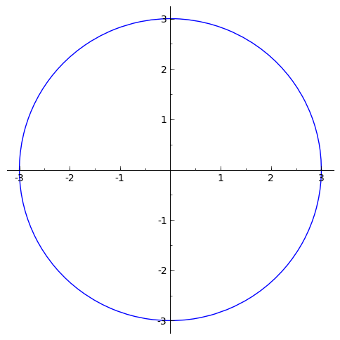
Circle of radius 3 centered at the origin

The default choice of aspect ratio makes the plot above decidedly “un-circle like”. We can adjust this by using the aspect_ratio option.

sage: p.show(aspect_ratio=1)

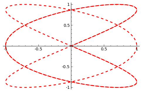
Circle of radius 3 with 1/1 aspect ratio

The different plotting commands accept many of the same options as plot. The following generates the Lissajous Curve $L(3,2)$ with a thick red dashed line.

sage: p = parametric_plot( [sin(3*t), sin(2*t)], (t, 0, 3*pi), thickness=2, color='red', linestyle="--")
sage: p.show()

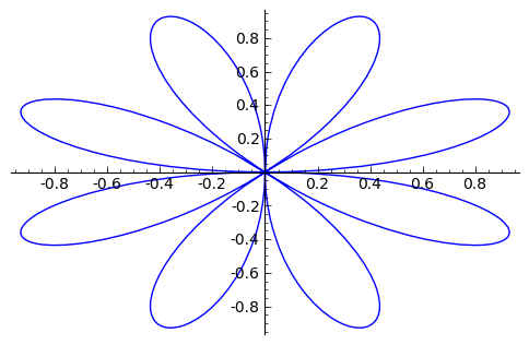
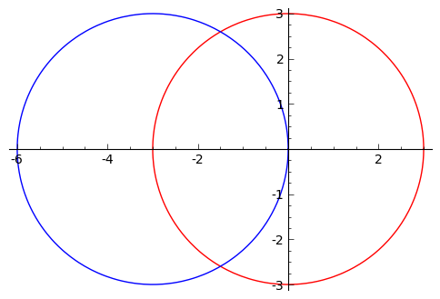
Polar plots can be done using the polar_plot() command.

sage: theta = var("theta")
sage: r(theta) = sin(4*theta)
sage: p = polar_plot((r(theta)), (theta, 0, 2*pi) )
sage: p.show()

And finally, Sage can do the plots for functions that are implicitly defined. For example, to display all points $(x,y)$ that satisfy the equation 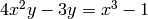$4x^2y - 3y = x^3 -1$ , we enter the following:

sage: implicit_plot(4*x^2*y - 3*y == x^3 - 1, (x,-10,10),(y,-10,10))

Example of plotting a curve defined implicitly

Exercises:

Plot the graph of $y = \sin\left(\pi x - \pi \right)$ for $-1 \leq x \leq 1$ using a thick red line.

Plot the graph of $\cos\left(\pi x - \pi \right)$ on the same interval using a thick blue line.

Plot the two graphs above on the same set of axes.

Plot the graph of $y = 1/x$ for $-1 \leq x \leq 1$ adjusting the range so that only $-10 \leq y \leq 10$ .

Use the commands in this section to produce the following image:

3D Graphics¶

Producing 3D plots can be done using the plot3d() command

sage: x,y = var("x y")
sage: f(x,y) = x^2 - y^2
sage: p = plot3d(f(x,y), (x,-10,10), (y,-10,10))
sage: p.show()

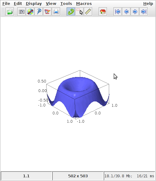
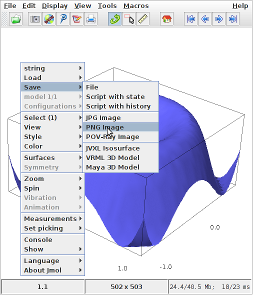
Sage handles 3d plotting a bit differently than what we have seen thus far. It uses a program named jmol to generate interactive plots. So instead of just a static picture we will see either a window like pictured above or, if you are using Sage’s notebook interface, a java applet in your browser’s window.

One nice thing about the way that Sage does this is that you can rotate your plot by just clicking on the surface and dragging it in the direction in which you would like for it to rotate. Zooming in/out can also be done by using your mouse’s wheel button (or two-finger vertical swipe on a mac). Once you have rotated and zoomed the plot to your liking, you can save the plot as a file. Do this by right-clicking anywhere in the window/applet and selecting save, then png-image as pictured below

Note

If you are running Sage on windows or on sagenb.org that your file will be saved either in your VMware virtual machine or on sagenb.org.

Sage as a Calculator¶

Arithmetic and Functions¶

Basic Arithmetic¶

Integer Division and Factoring¶

Standard Functions and Constants¶

Solving Equations and Inequalities¶

Solving for x¶

Declaring Variables¶

Solving Equations with Several Variables¶

Calculus¶

Limits¶

Derivatives¶

Integrals¶

Statistics¶

Plotting¶

2D Graphics¶

3D Graphics¶

Topics

This Page

Navigation

Sage as a Calculator¶

Arithmetic and Functions¶

Basic Arithmetic¶

Integer Division and Factoring¶

Standard Functions and Constants¶

Solving Equations and Inequalities¶

Solving for x¶

Declaring Variables¶

Solving Equations with Several Variables¶

Calculus¶

Limits¶

Derivatives¶

Integrals¶

Statistics¶

Plotting¶

2D Graphics¶

3D Graphics¶

Topics

This Page

Quick search